In this blog post, we will learn to partition graphs by spectral decomposition.

Blog Post 2: Spectral Clustering

In this blog, we will use the notation below for math expressions.

Notation

In all the math below:

• Boldface capital letters like \(\mathbf{A}\) refer to matrices (2d arrays of numbers).
• Boldface lowercase letters like \(\mathbf{v}\) refer to vectors (1d arrays of numbers).
• \(\mathbf{A}\mathbf{B}\) refers to a matrix-matrix product (A@B). \(\mathbf{A}\mathbf{v}\) refers to a matrix-vector product (A@v).

Introduction

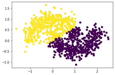
Clustering refers to the task of separating this data set into the two natural “blobs.” K-means is a very common way to achieve this task．Recall that k-means algorithm partitions observations by minimizing the within-cluster sum of squares. This algorithm works effectively in many cases, especially on circular-ish blobs, for example:

import numpy as np
from sklearn import datasets
from matplotlib import pyplot as plt

n = 200
np.random.seed(1111)
X, y = datasets.make_blobs(n_samples=n, shuffle=True, random_state=None, centers = 2, cluster_std = 2.0)
plt.scatter(X[:,0], X[:,1])

<matplotlib.collections.PathCollection at 0x24a1cef3f70>

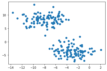
Now we have two circular-ish blobs that have clear separation. In situations like this, K-means algorithm can easily determine the clusters.

from sklearn.cluster import KMeans
km = KMeans(n_clusters = 2)
km.fit(X)

plt.scatter(X[:,0], X[:,1], c = km.predict(X))

<matplotlib.collections.PathCollection at 0x24a1ec59880>

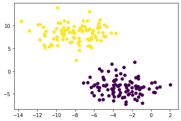
Now two clusters are colorred differently by K-means algorithm. As we can see, this gives us the correct clusters.

Harder Clustering

However, when our data is “shaped weird”, k-means clustering might not work so well. In the following example, we will create clusters that are shaped as crescents using make_moons() function from module datasets.

np.random.seed(1234)
n = 200
X, y = datasets.make_moons(n_samples=n, shuffle=True, noise=0.05, random_state=None)
plt.scatter(X[:,0], X[:,1])

<matplotlib.collections.PathCollection at 0x24a1ecc9d00>

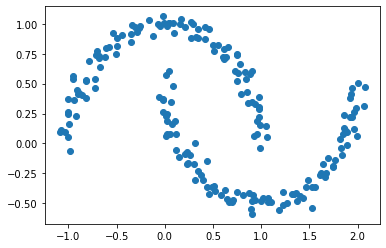
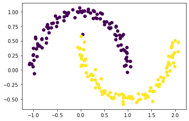
We can still make out two meaningful clusters in the data, but now they aren’t blobs but crescents. As before, the Euclidean coordinates of the data points are contained in the matrix X, while the labels of each point are contained in y. Now k-means won’t work so well, because k-means is, by design, looking for circular clusters.

km = KMeans(n_clusters = 2)
km.fit(X)
plt.scatter(X[:,0], X[:,1], c = km.predict(X))

<matplotlib.collections.PathCollection at 0x24a1ed32d30>

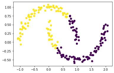
Whoops! That’s not right! K-means algorithm is not sufficient to correctly cluster our data in this case.

To resolve this problem, we’ll study spectral clustering, an important tool for identifying meaningful parts of data sets with complex structure. As we’ll see, spectral clustering is able to correctly cluster the two crescents. We will derive and implement spectral clustering in the following section.

Part A: Similarity Matrix

In multivariate statistics, spectral clustering techniques make use of the spectrum (eigenvalues) of the similarity matrix of the data to perform dimensionality reduction before clustering in fewer dimensions. The similarity matrix is provided as an input and consists of a quantitative assessment of the relative similarity of each pair of points in the dataset.

So, let’s construct the similarity matrix \(\mathbf{A}\). \(\mathbf{A}\) should be a matrix (2d np.ndarray) with shape (n, n) (recall that n is the number of data points).

When constructing the similarity matrix, we’ll use a parameter epsilon. Entry A[i,j] should be equal to 1 if X[i] (the coordinates of data point i) is within distance epsilon of X[j] (the coordinates of data point j), else it should be 0.

The diagonal entries A[i,i] should all be equal to zero.

euclidean_distance() is a nice function from sklearn.metrics.pairwise package that can help us easily compute the pairwise distance of a matrix.

from sklearn.metrics.pairwise import euclidean_distances
epsilon = 0.4
D = euclidean_distances(X) # pairwise distance matrix of X

# if distance smaller than epsilon, fill 1(true), otherwise 0 (false)
A = 1*(D< epsilon*np.ones(shape=(n,n)))

# update the diagonal entries to be 0
np.fill_diagonal(A,0)
A

array([[0, 0, 0, ..., 0, 0, 0],
       [0, 0, 0, ..., 0, 0, 0],
       [0, 0, 0, ..., 0, 1, 0],
       ...,
       [0, 0, 0, ..., 0, 1, 1],
       [0, 0, 1, ..., 1, 0, 1],
       [0, 0, 0, ..., 1, 1, 0]])

Part B: Partition

The matrix A now contains information about which points are near (within distance epsilon) which other points. We now pose the task of clustering the data points in X as the task of partitioning the rows and columns of A.

Let \(d_i = \sum_{j = 1}^n a_{ij}\) be the \(i\)th row-sum of \(\mathbf{A}\), which is also called the degree of \(i\). Let \(C_0\) and \(C_1\) be two clusters of the data points. We assume that every data point is in either \(C_0\) or \(C_1\). The cluster membership as being specified by y. We think of y[i] as being the label of point i. So, if y[i] = 1, then point i (and therefore row $i$ of \(\mathbf{A}\)) is an element of cluster \(C_1\).

The binary norm cut objective of a matrix \(\mathbf{A}\) is the function

In this expression,

• \(\mathbf{cut}(C_0, C_1) \equiv \sum_{i \in C_0, j \in C_1} a_{ij}\) is the cut of the clusters \(C_0\) and \(C_1\).
• \(\mathbf{vol}(C_0) \equiv \sum_{i \in C_0}d_i\), where \(d_i = \sum_{j = 1}^n a_{ij}\) is the degree of row \(i\) (the total number of all other rows related to row \(i\) through \(A\)). The volume of cluster \(C_0\) is a measure of the size of the cluster.

A pair of clusters \(C_0\) and \(C_1\) is considered to be a “good” partition of the data when \(N_{\mathbf{A}}(C_0, C_1)\) is small. To see why, let’s look at each of the two factors in this objective function separately.

B.1 The Cut Term

First, the cut term \(\mathbf{cut}(C_0, C_1)\) is the number of nonzero entries in \(\mathbf{A}\) that relate points in cluster \(C_0\) to points in cluster \(C_1\). Saying that this term should be small is the same as saying that points in \(C_0\) shouldn’t usually be very close to points in \(C_1\).

In the block below, we will write a function called cut(A,y) to compute the cut term by summing up the entries A[i,j] for each pair of points (i,j) in different clusters.

def cut(A,y):
    sum_cluster = 0
    
    for i in range(len(y)):
        for j in range(len(y)): 
            if y[i] != y[j]: # add all entries of A that has same corresponding y value
                sum_cluster += A[i][j]
    return(sum_cluster)

Compute the cut objective for the true clusters y. Then, generate a random vector of random labels of length n, with each label equal to either 0 or 1. Check the cut objective for the random labels. You should find that the cut objective for the true labels is much smaller than the cut objective for the random labels.

This shows that this part of the cut objective indeed favors the true clusters over the random ones.

temp = np.random.randint(2,size = n)
actual = cut(A,y) # the true clusters 
rand = cut(A,temp) # the randdom clusters
(actual,rand)

(26, 2300)

Indeed, the cut of true clusters is much smaller!

B.2 The Volume Term

Now take a look at the second factor in the norm cut objective. This is the volume term. As mentioned above, the volume of cluster \(C_0\) is a measure of how “big” cluster \(C_0\) is. If we choose cluster \(C_0\) to be small, then \(\mathbf{vol}(C_0)\) will be small and \(\frac{1}{\mathbf{vol}(C_0)}\) will be large, leading to an undesirable higher objective value.

Synthesizing, the binary normcut objective asks us to find clusters \(C_0\) and \(C_1\) such that:

1. There are relatively few entries of \(\mathbf{A}\) that join \(C_0\) and \(C_1\).
2. Neither \(C_0\) and \(C_1\) are too small.

We’ll write a function called vols(A,y) which computes the volumes of \(C_0\) and \(C_1\), returning them as a tuple. For example, v0, v1 = vols(A,y) should result in v0 holding the volume of cluster 0 and v1 holding the volume of cluster 1. Then, write a function called normcut(A,y) which uses cut(A,y) and vols(A,y) to compute the binary normalized cut objective of a matrix A with clustering vector y.

def vols(A,y):
    v0 = A[y == 0].sum() # row sum for which y == 0
    v1 = A[y == 1].sum() # row sum for which y == 1
    return(v0,v1)

def normcut(A,y):
    (v0,v1) = vols(A,y)
    c = cut(A,y)
    return(c*(1/v0+1/v1))

Now, compare the normcut objective using both the true labels y and the fake labels you generated above. What do you observe about the normcut for the true labels when compared to the normcut for the fake labels?

(normcut(A,y),normcut(A,temp))

(0.02303682466323045, 2.0480047195518316)

The true labels are much smaller.

Part C Transformation

We have now defined a normalized cut objective which takes small values when the input clusters are (a) joined by relatively few entries in \(A\) and (b) not too small. One approach to clustering is to try to find a cluster vector y such that normcut(A,y) is small. However, this is an NP-hard combinatorial optimization problem, which means that may not be possible to find the best clustering in practical time, even for relatively small data sets. We need a math trick!

Here’s the trick: define a new vector \(\mathbf{z} \in \mathbb{R}^n\) such that:

Note that the signs of the elements of \(\mathbf{z}\) contain all the information from \(\mathbf{y}\): if \(i\) is in cluster \(C_0\), then \(y_i = 0\) and \(z_i > 0\).

Next, if you like linear algebra, you can show that

where \(\mathbf{D}\) is the diagonal matrix with nonzero entries \(d_{ii} = d_i\), and where \(d_i = \sum_{j = 1}^n a_i\) is the degree (row-sum) from before.

1. Write a function called transform(A,y) to compute the appropriate \(\mathbf{z}\) vector given A and y, using the formula above.
2. Then, check the equation above that relates the matrix product to the normcut objective, by computing each side separately and checking that they are equal.
3. While you’re here, also check the identity \(\mathbf{z}^T\mathbf{D}\mathbb{1} = 0\), where \(\mathbb{1}\) is the vector of n ones (i.e. np.ones(n)). This identity effectively says that \(\mathbf{z}\) should contain roughly as many positive as negative entries.

Note

The equation above is exact, but computer arithmetic is not! np.isclose(a,b) is a good way to check if a is “close” to b, in the sense that they differ by less than the smallest amount that the computer is (by default) able to quantify.

# compute vector z
def transform(A,y):
    (v0,v1) = vols(A,y)
    # entries in z is 1/v0 when y==0, else is -1/v1
    z = 1/v0*(y == 0)-1/v1*(y == 1)
    return(z)

# check if the two approaches are equivalent
z = transform(A,y)
# compute the row sum
v = A.sum(axis = 1)
# row sum as the diagonal entries
D = np.diag(v)

np.isclose(normcut(A,y),2*z.T@(D-A)@z/(z.T@D@z))

True

# verify if z is evenly distributed between positive and negative entries
np.isclose(0,z.T@D@np.ones(n))

True

Part D: Minimization

In the last part, we saw that the problem of minimizing the normcut objective is mathematically related to the problem of minimizing the function

subject to the condition \(\mathbf{z}^T\mathbf{D}\mathbb{1} = 0\). It’s actually possible to bake this condition into the optimization, by substituting for \(\mathbf{z}\) the orthogonal complement of \(\mathbf{z}\) relative to \(\mathbf{D}\mathbf{1}\). In the code below, I define an orth_obj function which handles this for you.

Use the minimize function from scipy.optimize to minimize the function orth_obj with respect to \(\mathbf{z}\). Note that this computation might take a little while. Explicit optimization can be pretty slow! Give the minimizing vector a name z_min.

def orth(u, v):
    return (u @ v) / (v @ v) * v

e = np.ones(n) 

d = D @ e

def orth_obj(z):
    z_o = z - orth(z, d)
    return (z_o @ (D - A) @ z_o)/(z_o @ D @ z_o)

import scipy.optimize
z_min = scipy.optimize.minimize(orth_obj,np.random.rand(n)).x

Note: there’s a cheat going on here! We originally specified that the entries of \(\mathbf{z}\) should take only one of two values (back in Part C), whereas now we’re allowing the entries to have any value! This means that we are no longer exactly optimizing the normcut objective, but rather an approximation. This cheat is so common that deserves a name: it is called the continuous relaxation of the normcut problem.

Part E: Results

Recall that, by design, only the sign of z_min[i] actually contains information about the cluster label of data point i. Plot the original data, using one color for points such that z_min[i] < 0 and another color for points such that z_min[i] >= 0.

Does it look like we came close to correctly clustering the data?

color = (z_min <0)
plt.scatter(X[:,0], X[:,1], c = color)

<matplotlib.collections.PathCollection at 0x24a210694f0>

We are very close to correctly clustering the data!

Part F: Fast Algorithm

Explicitly optimizing the orthogonal objective is way too slow to be practical. If spectral clustering required that we do this each time, no one would use it.

The reason that spectral clustering actually matters, and indeed the reason that spectral clustering is called spectral clustering, is that we can actually solve the problem from Part E using eigenvalues and eigenvectors of matrices.

Recall that what we would like to do is minimize the function

with respect to \(\mathbf{z}\), subject to the condition \(\mathbf{z}^T\mathbf{D}\mathbb{1} = 0\).

The Rayleigh-Ritz Theorem states that the minimizing \(\mathbf{z}\) must be the solution with smallest eigenvalue of the generalized eigenvalue problem

which is equivalent to the standard eigenvalue problem

Why is this helpful? Well, \(\mathbb{1}\) is actually the eigenvector with smallest eigenvalue of the matrix \(\mathbf{D}^{-1}(\mathbf{D} - \mathbf{A})\).

So, the vector \(\mathbf{z}\) that we want must be the eigenvector with the second-smallest eigenvalue.

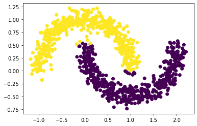
Construct the matrix \(\mathbf{L} = \mathbf{D}^{-1}(\mathbf{D} - \mathbf{A})\), which is often called the (normalized) Laplacian matrix of the similarity matrix \(\mathbf{A}\). Find the eigenvector corresponding to its second-smallest eigenvalue, and call it z_eig. Then, plot the data again, using the sign of z_eig as the color. How did we do?

L = np.linalg.inv(D)@(D-A)
Lam, U = np.linalg.eig(L)
ix = Lam.argsort()
Lam, U = Lam[ix], U[:,ix]
z_eig =  U[:,1]

plt.scatter(X[:,0], X[:,1], c = np.sign(z_eig))

<matplotlib.collections.PathCollection at 0x24a1fe92670>

In fact, z_eig should be proportional to z_min, although this won’t be exact because minimization has limited precision by default.Inspecting the scatterplot, z_eig gives us a really good estimation of clustering!

Part G: Summary

Now, Synthesize our results from the previous parts. In particular, write a function called spectral_clustering(X, epsilon) which takes in the input data X (in the same format as Part A) and the distance threshold epsilon and performs spectral clustering, returning an array of binary labels indicating whether data point i is in group 0 or group 1. Demonstrate your function using the supplied data from the beginning of the problem.

Outline

1. Construct the similarity matrix.
2. Construct the Laplacian matrix.
3. Compute the eigenvector with second-smallest eigenvalue of the Laplacian matrix.
4. Return labels based on this eigenvector.

def spectral_clustering(X, epsilon):
    '''
    this function computes the label for spectral clustering
    input: array X - the data that we want to perform spectral cluster on
           float epsion - the precision desired
    output: an array indicate the clusters each data point belongs to
    '''
    # construct similar matrix A
    n = len(X)
    A = 1*(euclidean_distances(X)< epsilon*np.ones(shape=n))
    np.fill_diagonal(A,0)
    
    # Laplacian matrix
    D = np.diag(A.sum(axis = 1))
    L = np.linalg.inv(D)@(D-A)
    
    # 2nd smalleset eigenvalue
    Lam, U = np.linalg.eig(L)
    ix = Lam.argsort()
    Lam, U = Lam[ix], U[:,ix]
    z_eig =  U[:,1]
    
    return(1*(z_eig>0))
    

spectral_clustering(X, epsilon)

array([1, 1, 0, 0, 0, 0, 0, 0, 1, 1, 1, 0, 0, 1, 1, 1, 1, 0, 0, 0, 1, 1,
       1, 0, 0, 1, 0, 1, 1, 0, 0, 1, 1, 1, 1, 1, 0, 1, 1, 0, 1, 0, 0, 0,
       0, 0, 0, 1, 1, 1, 0, 0, 1, 1, 0, 0, 1, 1, 1, 0, 0, 0, 1, 0, 1, 0,
       0, 0, 0, 1, 1, 1, 1, 0, 0, 0, 1, 0, 1, 0, 0, 0, 0, 1, 1, 1, 1, 0,
       0, 0, 0, 1, 0, 0, 1, 1, 1, 1, 0, 0, 1, 1, 1, 0, 1, 1, 0, 0, 1, 1,
       0, 0, 0, 1, 0, 0, 0, 0, 1, 1, 1, 0, 1, 1, 1, 0, 1, 0, 1, 1, 0, 0,
       0, 0, 1, 1, 1, 1, 1, 1, 1, 1, 0, 0, 1, 0, 0, 0, 0, 0, 0, 0, 0, 1,
       1, 0, 1, 0, 0, 0, 1, 1, 0, 0, 1, 1, 1, 0, 0, 0, 1, 0, 1, 1, 1, 0,
       0, 0, 0, 1, 1, 0, 0, 1, 1, 1, 0, 1, 1, 1, 0, 1, 0, 1, 1, 1, 1, 0,
       0, 0])

plt.scatter(X[:,0], X[:,1], c = spectral_clustering(X, epsilon))

<matplotlib.collections.PathCollection at 0x24a1fefedc0>

It looks like our function works! But let’s try a few more different instances.

Part H: Exploring Parameter Noise

Run a few experiments using your function, by generating different data sets using make_moons. What happens when you increase the noise? Does spectral clustering still find the two half-moon clusters? For these experiments, you may find it useful to increase n to 1000 or so – we can do this now, because of our fast algorithm!

X_test, y_test = datasets.make_moons(n_samples=1000, shuffle=True, noise=0.1, random_state=None)
label = spectral_clustering(X_test, epsilon)
plt.scatter(X_test[:,0], X_test[:,1], c = label)

<matplotlib.collections.PathCollection at 0x24a1f1fe370>

Our function works pretty well for noise = 0.1

X_test2, y_test2 = datasets.make_moons(n_samples=1000, shuffle=True, noise=0.2, random_state=None)
label = spectral_clustering(X_test2, epsilon)
plt.scatter(X_test2[:,0], X_test2[:,1], c = label)

<matplotlib.collections.PathCollection at 0x24a1f2702b0>

Well, it looks like our function doesn’t work so well for noise = 0.

Part I: Extension

Now try your spectral clustering function on another data set – the bull’s eye!

n = 1000
X, y = datasets.make_circles(n_samples=n, shuffle=True, noise=0.05, random_state=None, factor = 0.4)
plt.scatter(X[:,0], X[:,1])

<matplotlib.collections.PathCollection at 0x24a1f2c7eb0>

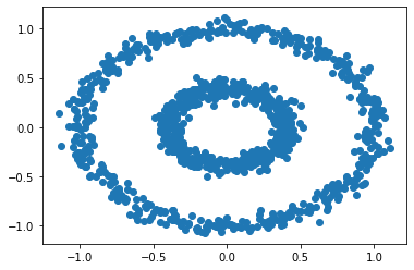
There are two concentric circles. As before k-means will not do well here at all.

km = KMeans(n_clusters = 2)
km.fit(X)
plt.scatter(X[:,0], X[:,1], c = km.predict(X))

<matplotlib.collections.PathCollection at 0x24a1f32c640>

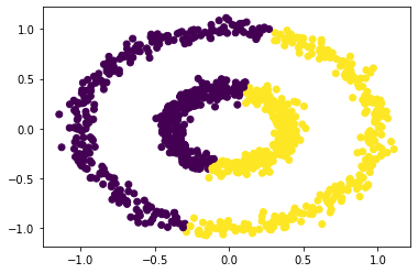
Can our function successfully separate the two circles?

epsilon = 0.3
label = spectral_clustering(X, epsilon)
plt.scatter(X[:,0], X[:,1], c = label)

<matplotlib.collections.PathCollection at 0x24a1f382ee0>

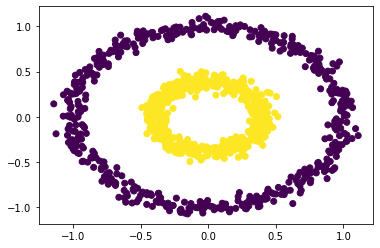
Isn’t this just amazing! Our function also correctly clustered two circles. What about larger epsilon values?

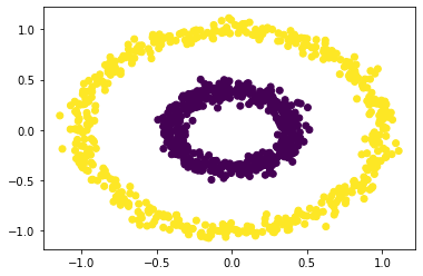
epsilon = 0.5
label = spectral_clustering(X, epsilon)
plt.scatter(X[:,0], X[:,1], c = label)

<matplotlib.collections.PathCollection at 0x2dae7b85df0>

epsilon = 0.6
label = spectral_clustering(X, epsilon)
plt.scatter(X[:,0], X[:,1], c = label)

<matplotlib.collections.PathCollection at 0x2dae7bea5e0>

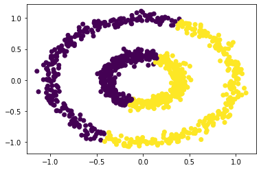
Our function can still correctly distinguish two rings when epsilon = 0.5, but when epsilon = 0.6, our function fails. Hence, wisely selecting the range of epsilon is essential for effective clustering.