
Blog Post 1 - Data Visualization with Matplotlib
In this blog post, we will explore Palmer’s Penguin dataset with multiple visualizations.
§0. Import Data
import pandas as pd
url = "https://raw.githubusercontent.com/PhilChodrow/PIC16B/master/datasets/palmer_penguins.csv"
penguins = pd.read_csv(url)
Let’s take a look at the first few rows of our data.
penguins.head()
| studyName | Sample Number | Species | Region | Island | Stage | Individual ID | Clutch Completion | Date Egg | Culmen Length (mm) | Culmen Depth (mm) | Flipper Length (mm) | Body Mass (g) | Sex | Delta 15 N (o/oo) | Delta 13 C (o/oo) | Comments | |
|---|---|---|---|---|---|---|---|---|---|---|---|---|---|---|---|---|---|
| 0 | PAL0708 | 1 | Adelie Penguin (Pygoscelis adeliae) | Anvers | Torgersen | Adult, 1 Egg Stage | N1A1 | Yes | 11/11/07 | 39.1 | 18.7 | 181.0 | 3750.0 | MALE | NaN | NaN | Not enough blood for isotopes. |
| 1 | PAL0708 | 2 | Adelie Penguin (Pygoscelis adeliae) | Anvers | Torgersen | Adult, 1 Egg Stage | N1A2 | Yes | 11/11/07 | 39.5 | 17.4 | 186.0 | 3800.0 | FEMALE | 8.94956 | -24.69454 | NaN |
| 2 | PAL0708 | 3 | Adelie Penguin (Pygoscelis adeliae) | Anvers | Torgersen | Adult, 1 Egg Stage | N2A1 | Yes | 11/16/07 | 40.3 | 18.0 | 195.0 | 3250.0 | FEMALE | 8.36821 | -25.33302 | NaN |
| 3 | PAL0708 | 4 | Adelie Penguin (Pygoscelis adeliae) | Anvers | Torgersen | Adult, 1 Egg Stage | N2A2 | Yes | 11/16/07 | NaN | NaN | NaN | NaN | NaN | NaN | NaN | Adult not sampled. |
| 4 | PAL0708 | 5 | Adelie Penguin (Pygoscelis adeliae) | Anvers | Torgersen | Adult, 1 Egg Stage | N3A1 | Yes | 11/16/07 | 36.7 | 19.3 | 193.0 | 3450.0 | FEMALE | 8.76651 | -25.32426 | NaN |
§1. Exploring Data
# shortern the species name
penguins["Species"] = penguins["Species"].str.split().str.get(0)
penguins.head()
| studyName | Sample Number | Species | Region | Island | Stage | Individual ID | Clutch Completion | Date Egg | Culmen Length (mm) | Culmen Depth (mm) | Flipper Length (mm) | Body Mass (g) | Sex | Delta 15 N (o/oo) | Delta 13 C (o/oo) | Comments | |
|---|---|---|---|---|---|---|---|---|---|---|---|---|---|---|---|---|---|
| 0 | PAL0708 | 1 | Adelie | Anvers | Torgersen | Adult, 1 Egg Stage | N1A1 | Yes | 11/11/07 | 39.1 | 18.7 | 181.0 | 3750.0 | MALE | NaN | NaN | Not enough blood for isotopes. |
| 1 | PAL0708 | 2 | Adelie | Anvers | Torgersen | Adult, 1 Egg Stage | N1A2 | Yes | 11/11/07 | 39.5 | 17.4 | 186.0 | 3800.0 | FEMALE | 8.94956 | -24.69454 | NaN |
| 2 | PAL0708 | 3 | Adelie | Anvers | Torgersen | Adult, 1 Egg Stage | N2A1 | Yes | 11/16/07 | 40.3 | 18.0 | 195.0 | 3250.0 | FEMALE | 8.36821 | -25.33302 | NaN |
| 3 | PAL0708 | 4 | Adelie | Anvers | Torgersen | Adult, 1 Egg Stage | N2A2 | Yes | 11/16/07 | NaN | NaN | NaN | NaN | NaN | NaN | NaN | Adult not sampled. |
| 4 | PAL0708 | 5 | Adelie | Anvers | Torgersen | Adult, 1 Egg Stage | N3A1 | Yes | 11/16/07 | 36.7 | 19.3 | 193.0 | 3450.0 | FEMALE | 8.76651 | -25.32426 | NaN |
To learn more about the relationships between penguin species and different features, we will write a function to see the different median values of different features among different species.
def penguin_summary_table(group_cols, value_cols):
    return penguins.groupby(group_cols)[value_cols].median().round(2)
penguin_summary_table(["Species", "Sex", "Island"],
                      ["Culmen Length (mm)", "Body Mass (g)",
                       "Culmen Depth (mm)", "Flipper Length (mm)"])
| Culmen Length (mm) | Body Mass (g) | Culmen Depth (mm) | Flipper Length (mm) | |||
|---|---|---|---|---|---|---|
| Species | Sex | Island | ||||
| Adelie | FEMALE | Biscoe | 37.75 | 3375.0 | 17.70 | 187.0 |
| Dream | 36.80 | 3400.0 | 17.80 | 188.0 | ||
| Torgersen | 37.60 | 3400.0 | 17.45 | 189.0 | ||
| MALE | Biscoe | 40.80 | 4000.0 | 18.90 | 191.0 | |
| Dream | 40.25 | 3987.5 | 18.65 | 190.5 | ||
| Torgersen | 41.10 | 4000.0 | 19.20 | 195.0 | ||
| Chinstrap | FEMALE | Dream | 46.30 | 3550.0 | 17.65 | 192.0 |
| MALE | Dream | 50.95 | 3950.0 | 19.30 | 200.5 | |
| Gentoo | . | Biscoe | 44.50 | 4875.0 | 15.70 | 217.0 |
| FEMALE | Biscoe | 45.50 | 4700.0 | 14.25 | 212.0 | |
| MALE | Biscoe | 49.50 | 5500.0 | 15.70 | 221.0 |
As shown in the table, only Adelie penguins live on Torgersen island. On Biscoe island, there are Gentoo and Adelie penguins. On Dream island, there are Chinstrap and Adelie penguins.
With respect to each species, the values for each feature for male and female don’t differ too much.
The culmen length of Adelie is significantly shorter than Chinstrap and Gentoo, and the body mass of Gentoo is significantly larger than Adelie and Chinstrap.
1.1 Inspect individual features with respect to species
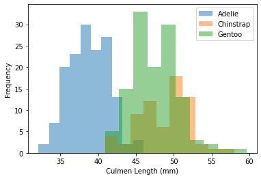
Let’s start from creating one histogram to compare the culmen length (mm) among different species. We can do do with hist function in the matplotlib package in python.
from matplotlib import pyplot as plt
for s in penguins["Species"].unique():
    # select the rows with species == s
    df = penguins[penguins["Species"] == s]
    # create histogram
    plt.hist(df["Culmen Length (mm)"], label = s, alpha = 0.5)

# add legend
plt.legend()

# add x-axis
plt.xlabel("Culmen Length (mm)")

# add y-axis
plt.ylabel("Frequency")
Text(0, 0.5, 'Frequency')
Great! Now, we can create histograms to visualize how Culmen Length (mm), Body Mass (g), Culmen Depth (mm), and Flipper Length (mm) values differ for each species of penguin in our data set.
fig, ax = plt.subplots(1,4, figsize = (13,3), sharey = True)
ax[0].set(ylabel = "Number of penguins")
features = ["Culmen Length (mm)", "Body Mass (g)",
            "Culmen Depth (mm)","Flipper Length (mm)"]

for i in range(0,len(features)):
    for s in penguins["Species"].unique():
        df = penguins[penguins["Species"] == s]
        ax[i].hist(df[features[i]], label = s, alpha = 0.3)
        ax[i].set(xlabel = features[i])

plt.tight_layout()
plt.legend()
<matplotlib.legend.Legend at 0x26128b416a0>
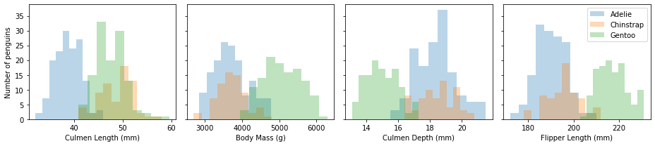
From the histograms, values of body mass, culmen length, and flipper length for Chinstrap penguins don’t differ much from those of Adelie penguins, but the culmen lengths for Chinstrap and Gentoo penguins are significantly different from those of Adelie penguins.
1.2 Inspect correlations between features
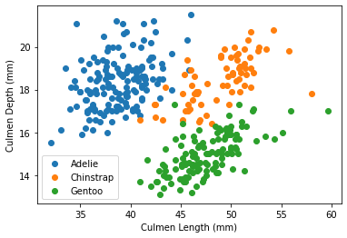
Now, we want to see if there’s some relationship between features. We can do so with the help of scatterplots. We can do do with scatter function in the matplotlib package in python.
First, let’s create a single scatterplot to observe the relationship between culmen length and culmen depth.
for s in penguins["Species"].unique():
    # select the rows with species == s
    df = penguins[penguins["Species"] == s]
    # create scatter
    plt.scatter(df["Culmen Length (mm)"], df["Culmen Depth (mm)"], label = s)

# add legend
plt.legend()

# add x-axis
plt.xlabel("Culmen Length (mm)")

# add y-axis
plt.ylabel("Culmen Depth (mm)")
Text(0, 0.5, 'Culmen Depth (mm)')
Now, we can create multiple scatterplots.
x = "Culmen Length (mm)"
y = ["Body Mass (g)", "Culmen Depth (mm)","Flipper Length (mm)"]
marker = {"Adelie"   : ".",
          "Chinstrap": "^",
          "Gentoo"   : "*"}
fig, ax = plt.subplots(1,3, figsize = (12,4))
for i in range(3):
    for s in penguins["Species"].unique():
        df = penguins[penguins["Species"] == s]
        ax[i].scatter(df[x], df[y[i]], label = s, marker = marker[s])
        ax[i].set(xlabel = x, ylabel = y[i])

plt.tight_layout()
plt.legend()
<matplotlib.legend.Legend at 0x2612adadf70>
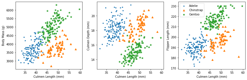
As we can see from the scatterplots, for Adelie, both body mass and flipper length are positively correlated with culmen length. For Chinstrap and Gentoo, all of body mass, culmen depth, and flipper length are positively correlated with culmen length.